ModelRisk
- Jul 6, 2025
- 8 min read
Updated: Jul 20, 2025
Estimating Oxygen Demand in a Bioreactor Using Monte Carlo Simulations from ModelRisk
Introduction
In this post I am going to focus on a wonderful, comprehensive, user-friendly Excel add-in called ModelRisk (www.vosesoftware.com) that allows you to easily fit probability distributions to data so you can conduct Monte Carlo simulations. Monte Carlo simulation is a probability method using repeated random sampling from a distribution to analyze the uncertainty in input variables that are then used to calculate an outcome or an output probability distribution.
Use ModelRisk to Replace Point Estimates
with Probability Distributions
The rate at which bacteria oxidize organics (measured as chemical oxygen demand [COD] or biochemical oxygen demand [BOD]), ammonia nitogen (NH3-N), and reduced sulfur compounds (bisulfide and hydrogen sulfide) and consume oxygen in an activated sludge bioreactor is highly variable. Maintaining a sufficient dissolved oxygen (DO) concentration of 2 to 3 mg/L in the bioreactor can be difficult and I see this frequently, particularly in heavily loaded and/or undersized industrial wastewater treatment plants.
For the purpose of this post, the two problems I want to solve using Monte Carlo simulations generated by ModelRisk, rather than point estimates, such as the mean, are:
Estimating the variable oxygen demand in a bioreactor given a range of wastewater flow rates, BOD loading rates (lb BOD/day), ammonia loading rates (lb NH3-N/day), and reduced sulfur loading rates (dissolved sulfide, lb/day).
When the oxygen demand in the bioreactor exceeds the oxygen generation capacity of the mechanical aeration system, I want to estimate how much hydrogen peroxide (gallons per day of a 50% H2O2 solution) would be required to provide supplemental DO.
The activated sludge system being evaluated has 470 horsepower (HP) of mechanical aeration installed and, in theory, should be able to supply between 22,925 to 35,837 pounds of oxygen per day to the bioreactor with a mean of 29,268 lb O2/d and a standard deviation of 1,685 lb O2/d. This is shown in the ModelRisk output histogram below.

Based on the available data and our knowledge of the wastewater system, input probability distributions are either fitted to data or chosen to closely match what we expect the possible range of values to be. My Excel/ModelRisk oxygen demand model includes 10 input variables and 10 output variables as shown below. The 10 input/10 output split is coincidence. You can have any number of variables as inputs and outputs in ModelRisk. The entire Excel model is shown (screenshots) at the end of this post.


Data Analysis and Data Exploration
One of my favorite activities in my job is working with wastewater laboratory data (process control data). Some data I generate myself doing very specific onsite testing (e.g., Oxygen Uptake Rate [OUR] and Adenosine Triphosphate [ATP]). Better still is getting comprehensive data from the customer that spans at least one or more years. A large dataset is going to require some degree of statistical analysis which, as an amateur statistician, is a hobby for me, providing many hours of enjoyable data analysis and data exploration, letting patterns and anomalies slowly reveal themselves as I work with the data.
Typically, the data starts in an Excel spreadsheet. After some (often a lot of!!) preliminary “data organizing and cleaning” I move to dedicated statistical analysis programs such as NCSS Statistical Software (www.ncss.com) and/or Minitab. The beginning of my data exploration is often a histogram with a normal curve fitted to the data, along with key, descriptive statistics, as shown below in the Summary Report, easily produced with Minitab.

The variable being evaluated in the summary report is the influent flow rate as measured from the final clarifier effluent flow meter (wastewater flow in = wastewater flow out) in units of gallons per minute (gpm). The dataset consists of 368 values with the average (mean) flow rate being 199 gpm, a median (middle value from the dataset) of 161 gpm, a standard deviation of 107 gpm, and a range of 455 gpm. The histogram has a long right tail (right or positive skewness) resulting in a poor fit for the normal curve. Shortly, we will easily correct this poor curve fit using ModelRisk's distribution fitting function.
A time series graph of the influent flow from Minitab is shown below followed by a tabulated summary of the data.

ModelRisk Distribution Fitting
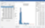
Using ModelRisk and Excel, we will fit an optimal probability distribution to the influent flow rate data. We will take our time, moving step-by-step to fit the distribution, which begins by selecting the data location in Excel, as shown in the top left of the ModelRisk screenshot below. The data location is simply the Excel spreadsheet column with the flow rate values.

Once we select the rows from the single column of data, ModelRisk generates a histogram, as shown below, similar to the histogram we saw above using Minitab. At this point I can enter minimum and maximum values before finding the best fitting distribution. These truncation values are optional and can be changed at any time. I used a minimum influent flow value of 94 and a maximum of 550 gpm.

The next step is to pick the type (or category) of distribution you want that you think best fits the type of data you have, as shown below. For the influent flow rate data, which can take on any random value between 94 and 550 gpm, I fit a continuous probability distribution.

As shown below, ModelRisk determined the best fit was a LogLaplace distribution, overlayed on the histogram, including shaded areas in both tails, matching the truncated values I entered. At this point you can move down through the distribution list, choosing any distribution you want, with the fit becoming less optimal the further down the list you go.
Having decided to use the best fitting LogLaplace distribution as determined by ModelRisk, I select the "Insert to Worksheet" button to add this to my Excel oxygen demand model in the Influent Flow cell which currently has a static or fixed value of 239 gpm as shown below.

In the Excel screenshot below, with the LogLaplace distribution entered into the Influent Flow cell, the flow value has increased to 324 gpm, changing from a static to a dynamic value due to the effect of the probability distribution and the fact that I have Excel formulas set to calculate automatically (see the Excel Options screenshot below).


ModelRisk Simulation with Input and Output Graph Results
To start a ModelRisk simulation, after identifying your input and output variables, you select the number of random samples you want to pull from all the inputs which will be used to generate a range of values for the outputs. You can see below I have selected 1,000 random samles for the simulation, with as many as 10,000 samples being an option. ModelRisk will generate a histogram for each input and output variable of which several examples will be shown below.

For the influent flow rate input distribution, after running 1,000 simulations, ModelRisk generated the histogram shown below. The mean influent flow rate is 188 gpm with a 90% liklihood the flow rate will range between 94 to 294 gpm, with a maximum flow of 522 gpm and a standard deviation of 76 gpm.

For the ModelRisk output variable of aeration horsepower required to meet the oxygen demand for the oxidation of BOD, ammonia, and reduced sulfur compounds, 470 HP is expected to be sufficient 86% of the time as shown in the histogram below. This means DO supplementation using hydrogen peroxide may be required 14% of the time.

Estimating the oxygen that can be supplied by mechanical aerators is tricky, at best. I've stated that 470 HP of mechanical aeration is available to supply oxygen to the bioreactor. This horsepower value alone is insufficient to properly (accurately) calculate oxygen input. Other factors that influence oxygen production from the aeration system include, but are not limited to, aerator placement in the bioreactor, water depth, air and water temperature, aerator oxygen transfer rate (see Excel/ModelRisk input range below), maintenance condition of the aerators, aerators in service at any given time, motor efficiency, etc.

Based on ModelRisk's simulation results, the mechanical aerator oxygen transfer rate is expected to range from 2.2 to 2.9 lb/O2/hp/hr 90% of the time, as shown in the histogram below. The mean of this histogram is 2.74 lb O2/hp/hr with a standard deviation of 0.14 lb O2/hp/hr.

I have several tables of aerator oxygen transfer data posted on another page which you can see by clicking on this link.
For those days when enough oxygen cannot be supplied by the aeration system, supplemental DO from hydrogen peroxide would require up to 2,007 gallons per day, covering 90% of low DO occurences as shown in the histogram below.

Tornado Chart
A nice feature provided by ModelRisk is the Tornado Chart, shown below, useful for doing sensitivity analysis on the input variables showing their impact on a specific output variable. For the pounds of oxygen required to oxidize BOD and ammonia, the Tornado chart shows us the influent flow has the largest impact, followed by the BOD and ammonia concentrations, all of which make a lot of sense.

Screenshots of the Complete Excel Oxygen Demand Model
The full oxygen demand model is shown below in a series of four screenshots placed close together. The colored cells are only intended to make it easier for me to navigate through the model. As you can see, the rows in light green are inputs to ModelRisk with rows in light grey representing outputs from ModelRisk. The light blue cells indicate calculation cells only and are not directly included in ModelRisk as an input or output.


ModelRisk References
Aven, Terje. Risk Analysis: Assessing Uncertainties Beyond Expected Values and Probabilities. Hoboken, NJ: John Wiley & Sons, 2009.
Evans, James R. and David L. Olson. Introduction to Simulation and Risk Analysis. Upper Saddle River, NJ: Prentice Hall, 1998.
Vose, David. Quantitative Risk Analysis: A Guide to Monte Carlo Simulation Modeling. New York, NY: John Wiley & Sons, 1996.
---. Risk Analysis: A Quantitative Guide. Third Edition. Hoboken, NJ: John Wiley & Sons, 2009.
In Closing
I have no affiliation with Vose Software. This is my second year of purchasing an annual, standalone license/subscription to use ModelRisk on a single computer. If I don't have something good to say about a software program, a textbook, a company or service, I will usually say nothing. But when I like something I tend to say a lot, as I have done in this post, because I want you to benefit just as I have. We are all different. In my case I find myself to be incredibly fascinated with modeling and simulation software and I cannot begin to count how many simulations I have run over the years. ModelRisk is a great piece of software, one I highly recommend, so I encourage you to try it out.